
Stephen F. O’Byrne, the President of Shareholder Value Advisors Inc., examines his intriguing research related to improved measures of pay for performance
U.S. companies now report a five-year history of Pay versus Performance in their proxy statements. The report has three highly informative disclosures: mark-to-market (MTM) pay for the CEO, company shareholder wealth, and peer company shareholder wealth. Still, it’s missing a critical piece of information: the CEO’s market pay. Once we have that missing piece, we can compare relative pay – that is, pay relative to opportunity cost – to relative performance and calculate four key pay dimensions: incentive strength, pay alignment, performance-adjusted cost, and relative pay risk.
Allocating market pay
In this report, we will explain how to estimate market pay and how to improve our pay dimension measures by allocating market pay to reflect the company’s utilization of opportunity cost. Allocating market pay to match resource allocation is important because a growing number of companies, including Apple, Alphabet, Palantir Technologies, and Tesla, have made large multi-year equity grants. At Palantir, CEO Alex Karp’s 2020 equity grant accounted for 98% of his 2020-2024 total pay. One recent study has found that 9% of companies used a front-loaded equity grant at least once between 1993 and 2022. (1)
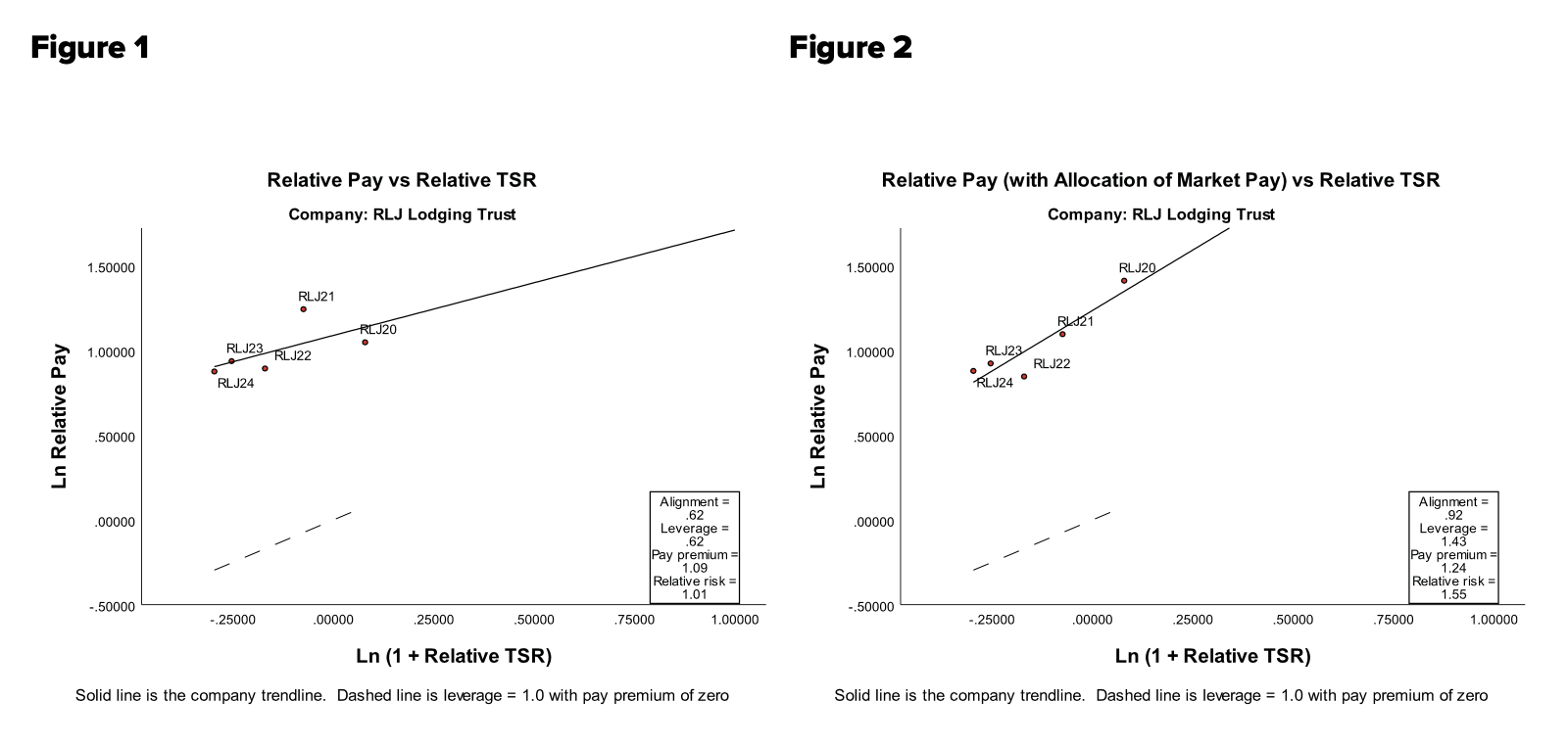
Before we explain how to estimate market rates and how to allocate the five-year market rate pool to match opportunity-cost usage, let’s take a look at how we estimate the four pay dimensions. Figure 1 shows our 2020-2024 pay leverage trendline for Leslie Hale, the CEO of RLJ Lodging Trust, a REIT that currently owns 95 hotels with more than 21,000 rooms. In this figure, there is no market pay allocation. The vertical axis is the natural log of relative pay, that is, cumulative MTM pay divided by cumulative market pay.
The horizontal axis is the natural log of [1 + relative TSR], that is, cumulative RLJ shareholder wealth divided by cumulative peer company shareholder wealth. The slope of the trendline, pay leverage, is a measure of incentive strength. Hale’s pay leverage of 0.62 means that a 1% increase in relative shareholder wealth increases her cumulative pay by only 0.62%. This puts her slightly below the 50th percentile of all U.S. companies. (2)
The correlation, 0.62 for Hale, is a measure of alignment. It tells us that relative TSR explains only 38% of the five-year variation in Hale’s relative pay. (3) The intercept, 1.09, is a measure of performance-adjusted cost. It’s the pay premium at industry average performance. It’s stated in logs, but we can convert it to a percent pay premium by taking the anti-log. Hale’s percentage pay premium at industry average performance is 197%. (4) This puts her above the 90th percentile of all U.S. companies. (5) The fourth pay dimension is relative pay risk, the ratio of relative pay variability to relative shareholder wealth variability.
Figure 2 shows the same graph with Hale’s market pay allocated to match the timing of her grant-date pay, which includes a large retention grant in 2021. The difference between Figure 2 and Figure 1 shows the importance of allocating market pay to match resource allocation. Pay leverage increases by 131% from 0.62 to 1.43, and alignment (r-sq) – the variance in relative pay explained by relative performance – increases by 124% from 38% to 85%.
Estimating and allocating market pay
Let’s now go back to the details of estimating and allocating market pay. The basic concept of market pay is average pay for executives in the same position in companies of similar size in the same industry. Size has a significant impact on executive pay. Studies dating back to the 1950s have found that doubling company size increases executive pay by 20-40%. (6) The leading proxy advisor, Institutional Shareholder Services (ISS), controls for size by limiting the data sample to 12-24 companies within a narrow size range of the subject company.
A better approach is to use regression analysis to control for size. Our estimate of 2020 market pay for Ms. Hale,
$3.3 million, is based on five years of inflation-adjusted pay data for CEOs in RLJ’s GICS industry, Hotel and Resort REITs. The sample is 49 CEO-years from 12 REITs. If we followed the ISS methodology and limited the sample to companies in the same year with revenue of 0.4 to 2.5 times RLJ’s revenue, we would have only eight observations (which ISS would increase to 12 by including companies from RLJ’s industry group, REITs).
Once we have our base-year market-rate estimate, we do two things to get an accurate estimate of pay leverage.
First, we don’t adjust our base year market rate for subsequent increases in sales. Adjusting for sales growth hides pay leverage because relative TSR is often correlated with sales growth.
For companies with 140%+ five-year sales growth, like RLJ, adjusting market pay for sales growth reduces mean pay leverage by almost 20%.
Second, we allocate market pay to years to reflect the company’s utilization of opportunity cost. Ms. Hale’s grant date pay jumps from $7.0 million in 2020 to $16.3 million in 2021 (when she received a special multi-year retention grant), then falls back to $8.4 million in 2022, $9.1 million in 2023, and
$9.4 million in 2024.
When we match the company’s utilization of grant-date pay (while keeping the present value of market pay the same), we get market pay of $2.3 million in 2020, $5.3 million in 2021, $2.7 million in 2022, $3.0 million in 2023, and $3.0 million in 2024. Matching market pay to reflect the company’s utilization of grant date pay increases Ms. Hale’s pay leverage by 129%, as Figure 2 shows.
References
- Copat, Rafael and Sunil Parupati, “Front-Loaded Equity Awards: An Efficient Contracting or Rent Extraction Tool?”, available at www.rafaelcopat.com/research.
- See Stephen F. O’Byrne, “Why and how U.S. executive pay should change”, Open Access Government, Figure 4.
- Alignment squared, 38% (= 0.62 x 0.62), is the variance explained.
- Exp(1.09)- 1 = 197%.
- Stephen F. O’Byrne, “Why and how U.S. executive pay should change”, Open Access Government, Figure 5.
- Patton, Arch (1995) “Building On the Executive Pay Survey”, Harvard Business Review, Vol 33, No 3, May/ June.


 Project")
